Advantages of geometric distance
The geometric distance detects the amount of "difference in peak frequency" and "difference in peak time".
- In the power spectrum of the voice, peaks called formants are observed. For the formant peaks, a “difference in peak frequency” and a “difference in peak time” occur for every utterance, even when the same voice is uttered.
- Figure 1A shows an example of the “difference” where the standard sound has two peaks in the spectrogram, and input sounds 1, 2 and 3 have a different position for the first peak. Note that both the standard and input sounds have the same volume.
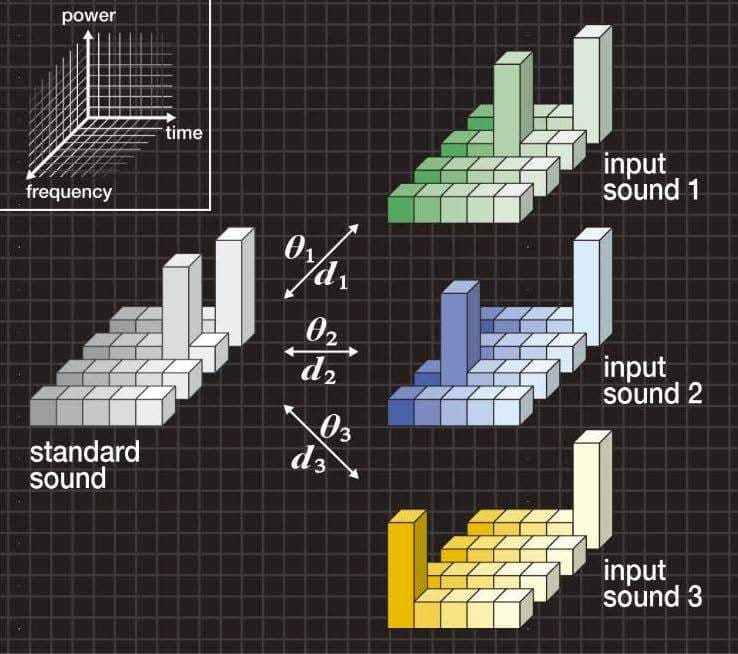
Figure 1A. Typical example of “difference in peak”
- In Figure 1B, the bar graph on the left shows the cosine similarities θ1, θ2 and θ3 between the standard sound and each of the input sounds 1, 2 and 3. Given that the cosine similarities have the relationship of θ1=θ2=θ3, and therefore, the input sounds 1, 2 and 3 cannot be distinguished from one another.
- In Figure 1B, the bar graph on the right shows the geometric distances d1, d2 and d3 between the standard sound and each of the input sounds 1, 2 and 3. The geometric distance can distinguish these three input sounds by detecting the amount of “difference in peak frequency” and “difference in peak time”.
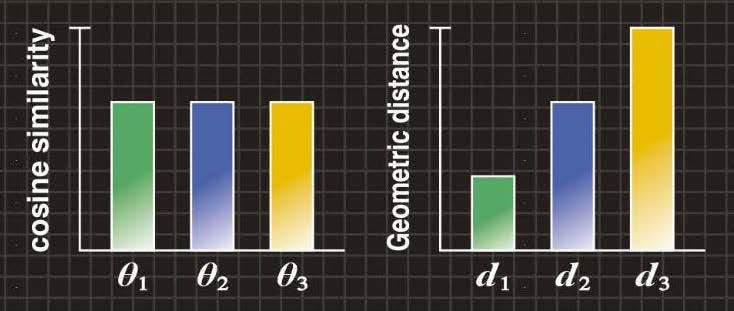
Figure 1B.Cosine similarity and geometric distance
Conventional cosine similarity
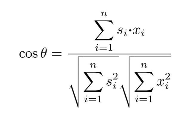
We create a standard pattern vector s having si (i = 1, 2, …, n) components of the standard image (or sound), and an input pattern vector x having xi (i = 1, 2, …, n) components of the input image (or sound), and represent them as follows.
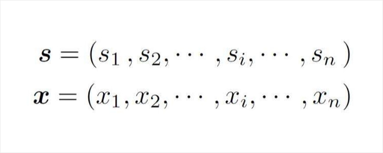
The cosine similarity is then calculated using the following equation. Note that Figures 1B-4B show the angle θ, which is calculated using an arccosine.
The geometric distance absorbs the "spectrum intensity wobble".
- A flat power spectrum is observed in spirant /s/. In the power spectrum of the spirant, a “spectrum intensity wobble” occurs for every utterance, even when the power spectrum form is flat.
- Figure 2A shows an example of the “wobble” where the standard sound has a flat spectrogram, input sounds 4 and 5 have the “wobble” on the flat spectrogram, and input sound 6 has a single peak. Each sound is assumed to have variable α, so the standard and input sounds always have the same volume.
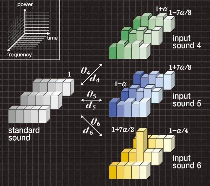
Figure 2A. Typical example of “wobble”
- In Figure 2B, the bar graph on the left shows the cosine similarities θ4, θ5 and θ6 between the standard sound and each of the input sounds 4, 5 and 6. The cosine similarities have the relationship of θ4=θ5=θ6, and therefore, the input sounds 4, 5 and 6 cannot be distinguished from one another.
- In Figure 2B, the bar graph on the right shows the geometric distances d4, d5 and d6 between the standard sound and each of the input sounds 4, 5 and 6. The geometric distance can distinguish the input sounds 4 and 5 from input sound 6 after absorbing the “spectrum intensity wobble”.
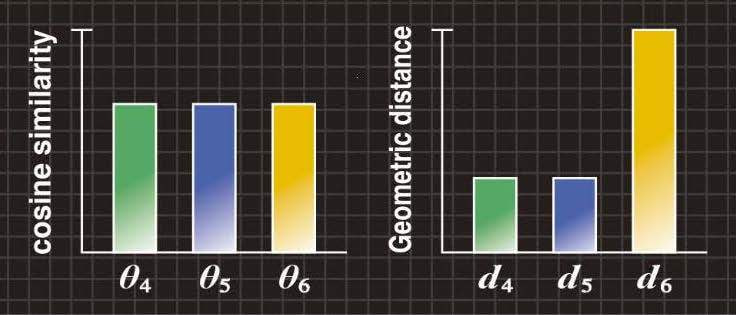
Figure 2B. Cosine similarity and geometric distance
The geometric distance detects the amount of "difference in position".
- With respect to image recognition, a “difference in position” of line occurs in every handwritten character, even when the same character is written.
- Figure 3A shows an example of the “difference in position” where the standard image has a symbol “+”, and input images 1, 2 and 3 have a different position on the horizontal bar.
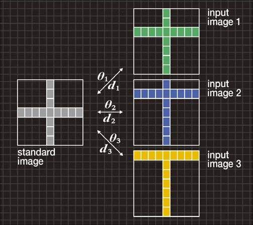
Figure 3A. Typical example of “difference in position”
- In Figure 3B, the bar graph on the left shows the cosine similarities θ1, θ2 and θ3 between the standard image and each of the input images 1, 2 and 3. The cosine similarities have the relationship of θ1=θ2=θ3, and therefore, input images 1, 2 and 3 cannot be distinguished from one another.
- In Figure 3B, the bar graph on the right shows the geometric distances d1, d2 and d3 between the standard image and each of the input images 1, 2 and 3. The geometric distance can distinguish these three input images by detecting the amount of “difference in position”.

Figure 3B. Cosine similarity and geometric distance
The geometric distance absorbs the "character deformation".
- “Character deformation” (changes in position and length of lines composing the character) occurs in every handwritten character, even when the same character is written.
- Figure 4A shows an example of “character deformation” where the standard image has the letter “E” and input images 4, 5 and 6 have the letters “E”, “F” and “G”, respectively.
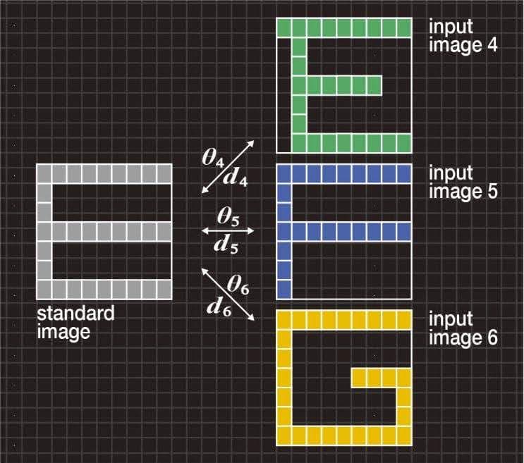
Figure 4A. Typical example of “character deformation”
- In Figure 4B, the bar graph on the left shows the cosine similarities θ4, θ5 and θ6 between the standard image and each of the input images 4, 5 and 6. The cosine similarities have the relationship of θ4>θ5>θ6, and therefore, the input letter “E” cannot be recognized correctly.
- In Figure 4B, the bar graph on the right shows the geometric distances d4, d5 and d6 between the standard image and each of the input images 4, 5 and 6. The geometric distance can recognize the letter “E” correctly after absorbing the "character deformation".
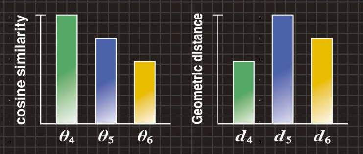
Figure 4B. Cosine similarity and geometric distance
Find the geometric distance between one-dimensional patterns.
- Figure 5 shows the momentary power spectrum of a machine sound. The geometric distance between the standard sound and the input sound can be obtained for sounds like this.
- The geometric distance detects the “spectrum intensity change” and the “difference in frequency” in the spectrum peak measurement despite the “spectrum intensity wobble” due to machine operation.
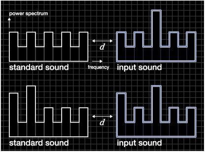
Figure 5. Typical example of “momentary power spectrum”
In the GD algorithm, when a “difference” occurs between peaks of the standard and input patterns with a “wobble” due to noise, the “wobble” is absorbed and the distance metric increases monotonically according to the increase of the “difference”.
Conventional similarity scales known as the Euclidean distance and cosine similarity compare the patterns using one-to-one mapping. The result of the one-to-one mapping is that the distance metric is highly sensitive to noise, and the distance metric changes in a staircase pattern when a difference occurs between peaks of the standard and input patterns.
The GD algorithm based on one-to-many point mapping is proposed to realize the human sense. In the GD algorithm, when a “difference” occurs between peaks of the standard and input patterns with a “wobble” due to noise, the “wobble” is absorbed and the distance metric increases monotonically according to the increase of the “difference”.
Principle of geometric distance
< Assumption of mathematical model >
A similarity scale is a concept that should concur intuitively with the human concept of similarity for hearing and sight. First we need to develop a mathematical model for the similarity scale so that we can perform numerical processing by computation. For GD, a mathematical model of similarity is proposed to improve the shortcomings that are found in the Euclidean distance, cosine similarity and others.
A mathematical model incorporating the following two characteristics is used.
A distance metric that shows good immunity to noise.
A distance metric that increases monotonically when a difference
increases between peaks of the standard and input patterns.
Bar graphs on the right of Figures 1B, 2B and 3B express the characteristics
andof the mathematical model.
< Development of algorithm >
A new algorithm based on a one-to-many point mapping is proposed to realize the mathematical model. In statistical analysis, a normal distribution is often used for models exhibiting many phenomena. Then, a "kurtosis" and a "skewness" are used to verify whether the phenomenon obeys the normal distribution or not. Here, the kurtosis and the skewness are statistics. With the GD algorithm, as shown in Figure 6, a difference δ in shapes between standard and input patterns is replaced by the shape change δ of the reference pattern having the shape of the normal distribution. For the reference pattern whose shape has changed, the magnitude of shape change is numerically evaluated as the variable of kurtosis and skewness.
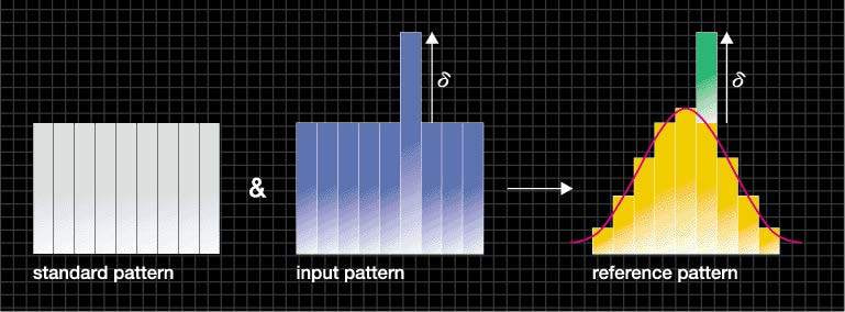
Figure 6. Standard pattern, input pattern and reference pattern
If a probability distribution of the phenomenon follows the normal distribution, then a = 3 (Figure 7(b)). If it has flatness relative to the normal distribution, then a <3 (Figure 7(a)). Conversely, if it has peakedness relative to the normal distribution, then a > 3 (Figure 7(c)).
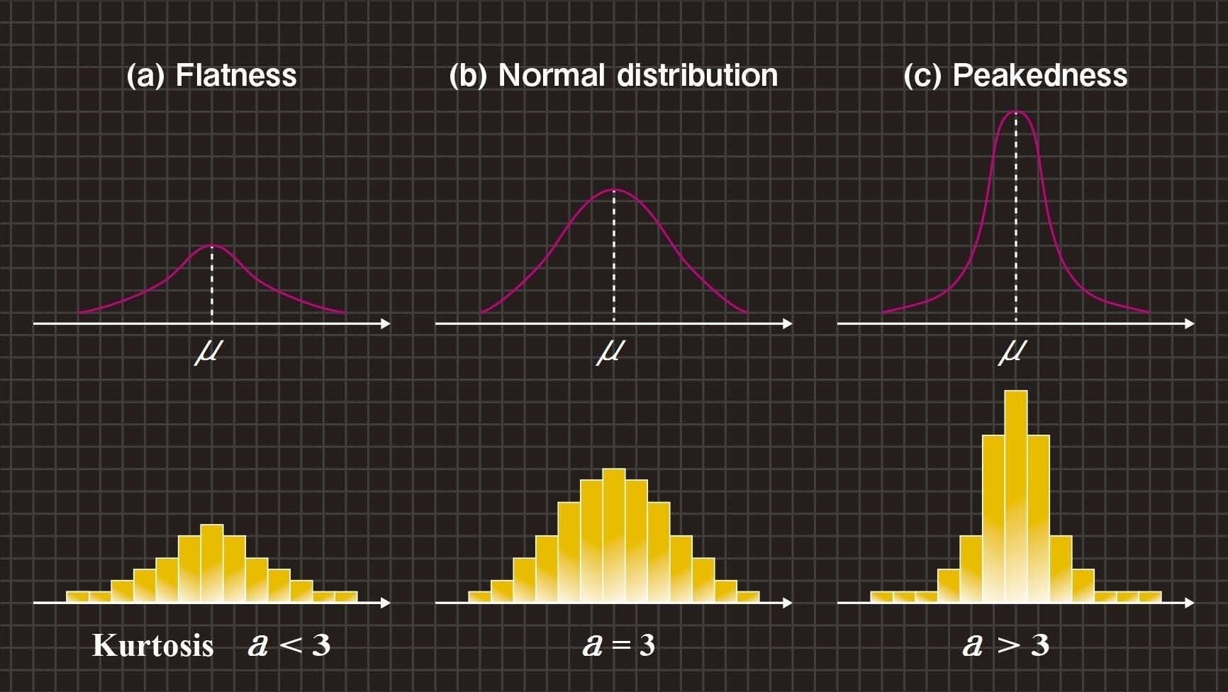
Figure 7. Shape change and kurtosis value ‘a’
Also, if a probability distribution of the phenomenon is symmetrical about the mean μ, then b = 0 (Figure 8(b)). If the tail on the left side of the probability distribution is longer than the right side, then b < 0 (Figure 8(a)). Conversely, if the tail on the right side of the probability distribution is longer than the left side, then b > 0 (Figure 8(c)).
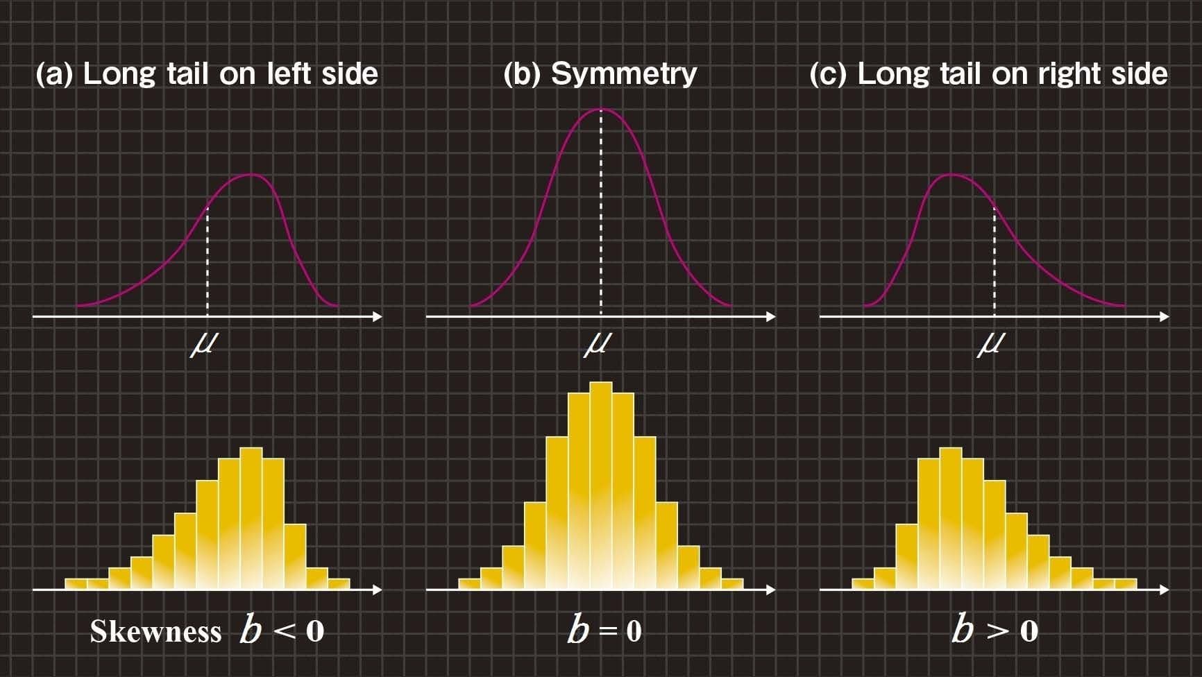
Figure 8. Shape change and skewness value ‘b’
In this section, we explain the GD algorithm using Figures 9 and 10.
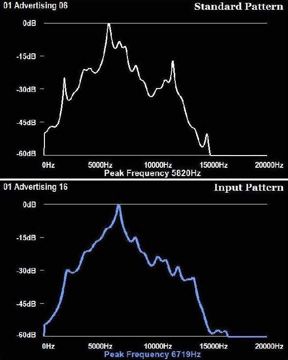
Figure 9. Standard and input patterns
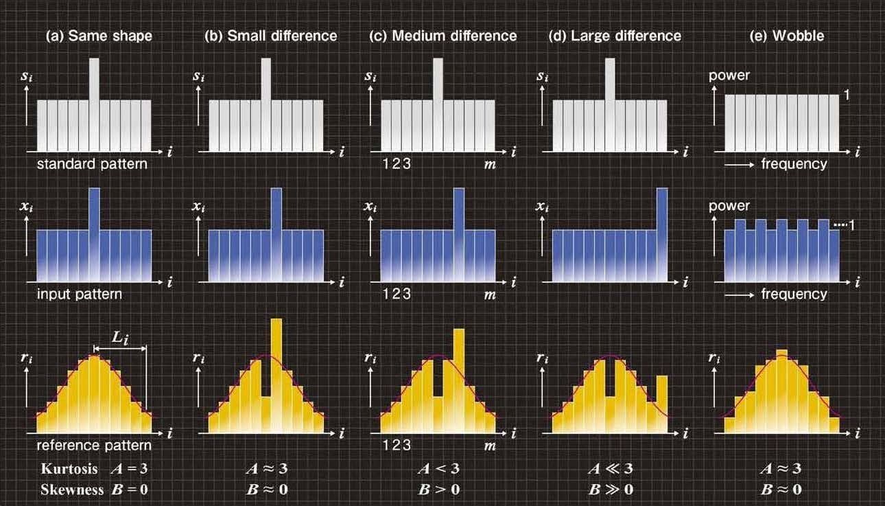
Figure 10. Shape change of reference patterns
Figure 9 shows the spectra (frequency-power) extracted from a Macleay’s Fig Parrot (Cyclopsitta diophthalma macleayana) vocalization. Figure 9 shows standard and input patterns that have been created using the momentary power spectrum (frequency-power) of standard and input sounds. Figures 10(a)-(e) respectively show typical examples of the standard and input patterns. Note that the power spectrum is generated from the output of a filter bank with m frequency bands. The i-th power spectrum values (where, i = 1, 2, … , m) of the standard and input sounds are divided by their total energy, so that normalized power spectra si and xi have been calculated, respectively. At this moment, the standard and input patterns have the same area size.
Here, we create a standard pattern vector s having si components, and an input pattern vector x having xi components, and represent them as Equation (1). Equation (1) expresses the shapes of the standard pattern and input pattern by the m pieces of component values of the pattern vector respectively.

(1)
Moreover, Figures 10(a)-(e) respectively show reference patterns that have the initial shape ri of a normal distribution. Here, we create a reference pattern vector r having ri components, and represent it as Equation (2). Equation (2) expresses the shape of the normal distribution by the m pieces of component values of the pattern vector.

(2)
With the GD algorithm, a difference in shapes between standard and input patterns is replaced by the shape change of the reference pattern using Equation (3).

(3)
Next, we explain Equation (3) using Figures 10(a)-(e).
Figure 10(a) gives an example of the case where the standard and input patterns have the same shape. Because values ri of Equation (3) do not change during this time, the reference pattern shown in Figure 10(a) does not change in the shape from the normal distribution.
Figures 10(b)-(d) respectively show examples exhibiting a small, medium, and large “difference” of peaks between the standard and input patterns. If Equation (3) is represented by the shapes, as shown in Figures 10(b)-(d), value ri decreases at peak position i of each standard pattern. At the same time, value ri increases at peak position i of each input pattern.
Figure 10(e) typically shows the standard pattern having a flat shape and the input pattern where a “wobble” occurs in the flat shape. Because values ri increase and decrease alternatively in Equation (3) during this time, the reference pattern shown in Figure 10(e) has a small shape change from the normal distribution.
With the GD algorithm, we replace the mean μ shown in Figures 7 and 8 with the center axis of the normal distribution (reference pattern) shown in Figure 10(a). Then, we replace the kurtosis ‘a’ and the skewness ‘b’ with a kurtosis ‘A’ and a skewness ‘B’ shown in Equations (4). Where, Li (i = 1, 2, … , m) is a deviation from the center axis of the normal distribution as shown in the reference pattern of Figure 10(a).

(4)
For the reference pattern whose shape has changed by Equation (3), the magnitude of shape change is numerically evaluated as the variable of kurtosis A and skewness B. The kurtosis and the skewness of the reference pattern can be calculated using Equations (4). Figures 10(a)-(e) show how A and B vary with ri.
In Figure 10(a), the values ri do not change. The kurtosis becomes A = 3 and the skewness becomes B = 0.
In Figure 10(b), the position i of the decreased ri and that of the increased ri are close. Because the effect of an increase and a decrease is cancelled out, the kurtosis becomes A ≈ 3 and the skewness becomes B ≈ 0.
In Figure 10(d), because the shape of the reference pattern is flattened relative to the normal distribution and the shape of the reference pattern has a long tail to the right side, the kurtosis becomes A << 3 and the skewness becomes B >> 0.
In Figure 10(c), because the shape of the reference pattern is an intermediate state between (b) and (d), the kurtosis becomes A < 3 and the skewness becomes B > 0.
In Figure 10(e), the reference pattern has small shape change from the normal distribution, and the kurtosis becomes A ≈ 3 and the skewness becomes B ≈ 0.
From Figures 10(a)-(d), we can understand that the values |A| and |B| respectively increase monotonically according to the increase of the “difference” between peaks of the standard and input patterns. Also, from Figures 10(e), it is clear that A ≈ 3 and B ≈ 0 for the “wobble”.
In this method, when a “difference” occurs between peaks of the standard and input patterns with a “wobble” due to noise, the “wobble” is absorbed and the distance metric increases monotonically purely in accord with the increase of the “difference”.
On this basis, we verify that the GD algorithm matches the characteristics and of the mathematical model.
< Evaluation experiments >
Refer to Paper No.10
To authenticate the effectiveness of the GD algorithm described above, we performed evaluation experiments for the vocalizations of Macleay’s Fig-Parrot.
Figure 11 shows that, using the GD algorithm, pattern matching even in a noisy environment is accurate.

Figure 11. Result of pattern matching for bird call recognition in a noisy environment
Refer to Paper No.12
The same GD algorithm has been successfully used to locate cavities in concrete structures by comparing the acoustic response to controlled surface tapping above integral concrete and concrete compromised by erosion cavities.
Figure 12 shows a measurement method of the sound generated by tapping a concrete test specimen with a hammer.
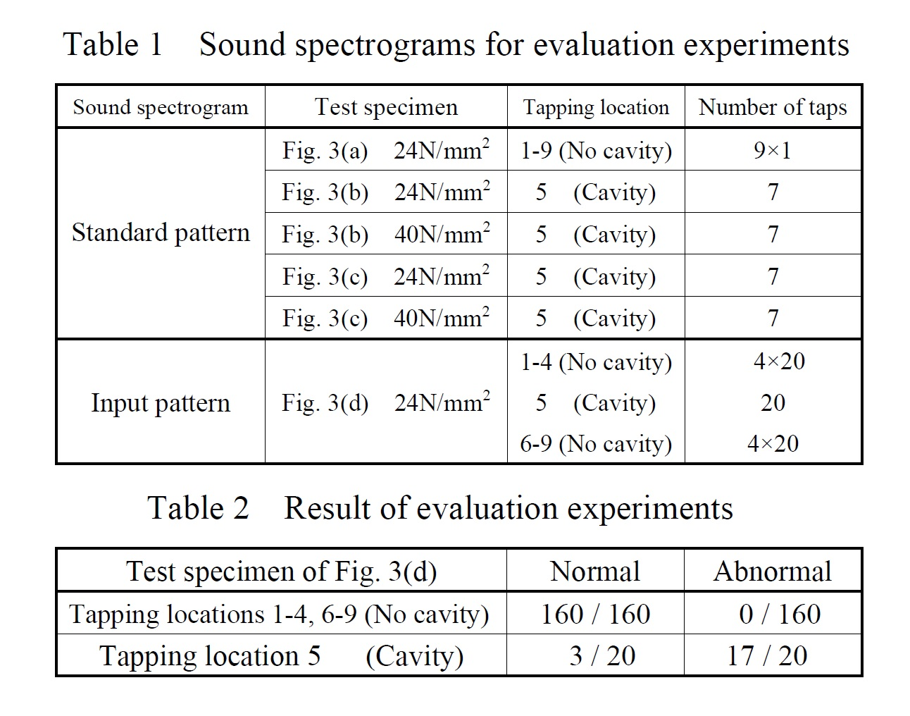
Table 1 shows the types of test specimens used for the standard and input patterns.
Table 2 shows the result of evaluation experiments. From Table 2, it is learned that the input sounds recorded at tapping locations 1-4 and 6-9, each beyond the cavity footprint, are recognized as ‘normal’ in all cases, and the recognition accuracy at tapping location 5 above cavities is 17/ 20. Thus we have verified the effectiveness of the GD algorithm.
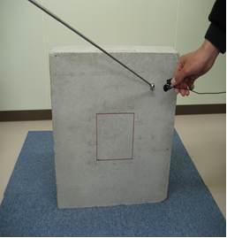
Figure 12. measurement method of vibrational response of concrete test specimen
Refer to Paper No.1
To confirm that the GD algorithm matches the mathematical model that we have assumed above, we performed numerical experiments to calculate the geometric distance between the standard and input patterns shown in Figures 1A and 2A.
From the numerical experiments, we could verify that the GD algorithm matches the characteristics <1> and <2> of the mathematical model.
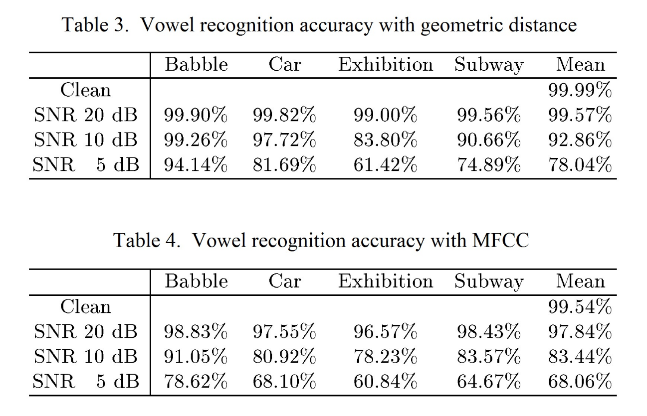
Experiments in speech vowel recognition were carried out under various SNR levels in a variety of noisy environments.
Tables 3 and 4 show the results of vowel recognition using the geometric distance and MFCC (Mel-Frequency Cepstrum Coefficients), respectively.
From these tables, it is learned that the recognition accuracy with the geometric distance is higher than that with the MFCC in all cases. In particular, “mean” of 10 dB and 5 dB SNR has improved approximately by 10%. Thus we confirm the effectiveness of the mathematical model and the GD algorithm.
