


The sound spectrum patterns are usually produced using the computationally efficient FFT. However, the upper spectrum of Figure 1 shows that the FFT generates much subtle detail that is largely redundant in recognition. Furthermore, because the FFT is ideal for long steady-state signals, it produces artifacts when applied to short sounds.
The LPC (Linear Predictive Coefficient) is much more suitable for such transient signals. The lower spectrum of Figure 1 shows that the LPC does not generate artifacts. Hence we have adopted the LPC, which, despite its computational complexity, is not an issue with today’s high-speed computers. The software executes 64-bit parallel processing using multiple CPUs.
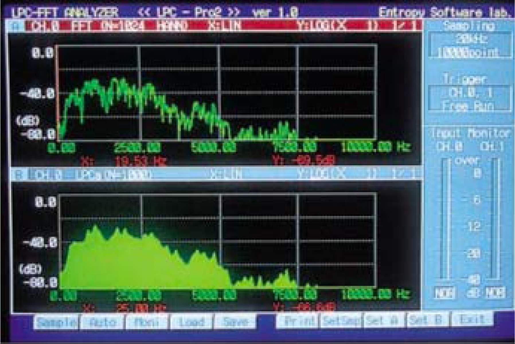
Figure 1. FFT spectrum (upper) and LPC spectrum (lower) analyzing machine noise
What is LPC(Linear Predictive Coefficient)spectrum analysis?
In 1967, Burg reported on a new spectrum analysis method called MEM(Maximum Entropy Method)for analysis of seismic waves. Because the MEM is able to obtain a high resolution spectrum from transient signals including seismic waves, MEM application has spread to the study of geomagnetic variations, solar cycles and voice recognition since the 1970s. It also goes by other names including AR(auto-regression)and LPC(Linear Predictive Coefficient)in these studies. The MEM, however, has not spread to other general fields due to the heavy calculation load that prevents realtime processing. However, the recent development of high-speed microprocessors has achieved LPC spectrum real-time processing, enabling the LPC spectrum analysis to be applied to many fields.

Figure 2. LPC spectrogram (upper) and oscillogram (lower) of bat call
Features of respective spectrum analyses
In the digital signal processing field, the following two spectrum analysis methods are famous; the FFT method reported in 1965 and the LPC method reported in 1967.
Features of FFT
Fast Fourier Transform
Calculations are small. The frequency resolution is ∆f =(1/T)Hz for waveform data length T seconds. The FFT is suitable for steady-state signals with long waveform data length T.
Features of LPC
Linear Predictive Coefficient
Frequency resolution ∆f can be specified regardless of the waveform data length T seconds. Calculations are large. The LPC is suitable for transient signals with short waveform data length T.
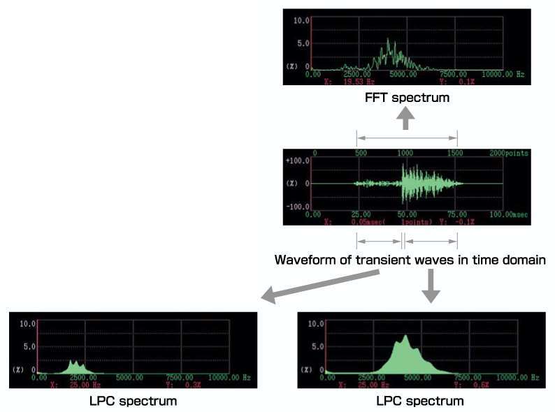
Figure 3. Transient waveform, FFT spectrum and LPC spectrum
LPC Spectrum Analyzer Software
We provide the spectrum analyzer software that displays LPC spectrum of various sounds including bird call, voice, impact sound, seismic wave and long steady-state signal. The software works on Microsoft Windows. First, you record the sounds into the WAV files using a data recorder. As shown in Figure 4, the software gives FIR digital filter processing to the waveform of sound (WAV file). Then, the software calculates “One-dimensional LPC spectrum”, “Two-dimensional LPC spectrum” and “Sonogram”.
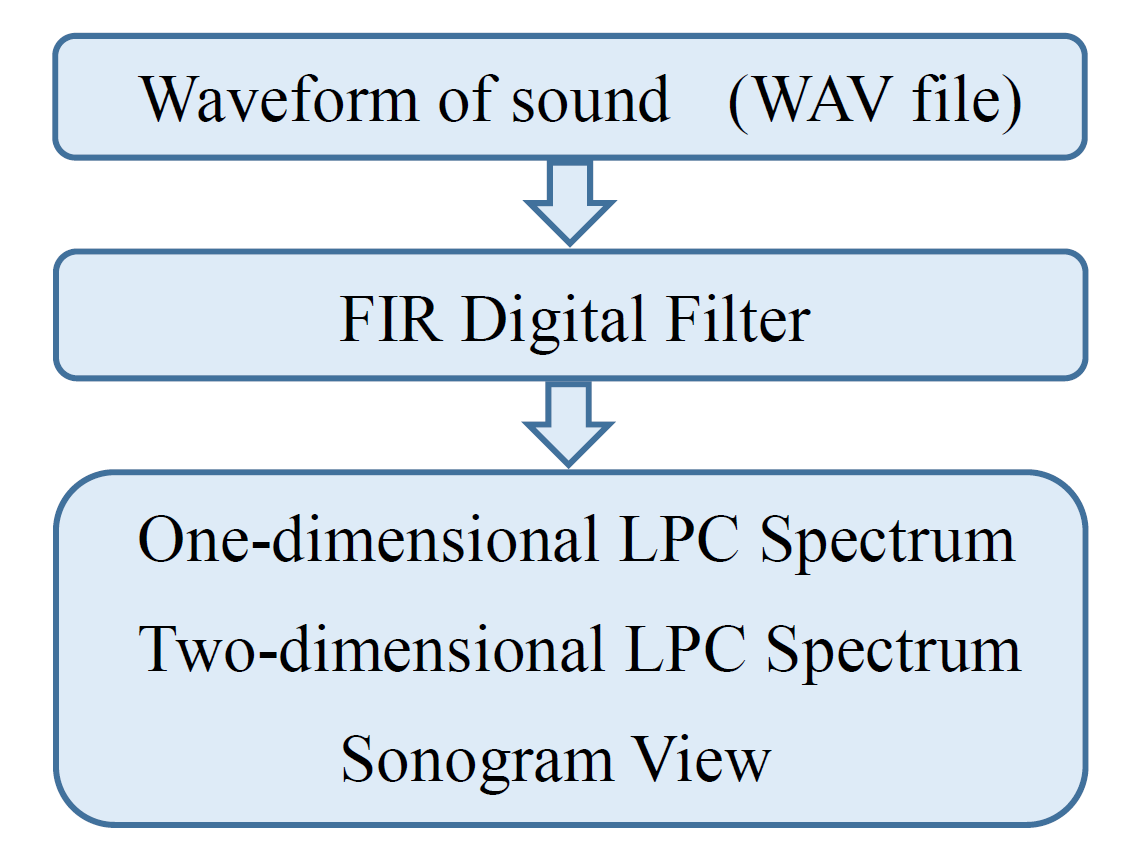
Figure 4. Processing procedure
LPC Spectrum Analyzer Program Menu
First, in the three RadioButtons at the bottom left of the menu screen shown in Figure 5, you click to select one from among ●Bird call or Voice (Transient signals) ●Concrete (Impact sounds) ●Machine (Steady-state signals). Then, the software segments waveforms of the target sound automatically from a continuous recording. Next, in the six Buttons at the top of the menu screen, you click to select one from among “LPC 1-d”, “LPC 2-d”, “Sonogram View” and other things. Then, the software displays “One-dimensional LPC spectrum”, “Two-dimensional LPC spectrum”, “Sonogram” and other things.
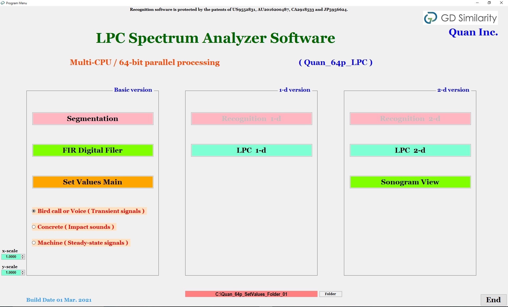
Figure 5. Program menu screen
LPC 1-d
At the top of the screen shown in Figure 6, the software displays the oscillogram and the one-dimensional LPC spectrum of the WAV file that is selected from the first cluster. Similarly, in the middle of the screen, the software displays the oscillogram and the one-dimensional LPC spectrum of the WAV file that is selected from the second cluster. Note that, the software displays the filtered oscillograms by the FIR digital filter, and extracts the one-dimensional LPC spectra from the cyan-colored waveforms, respectively. We can compare the one-dimensional LPC spectrum shown at the top of the screen with the one-dimensional LPC spectrum shown in the middle of the screen. Furthermore, at the bottom of the screen, the software displays the list of the peak frequencies in the one-dimensional LPC spectra of all WAV files.
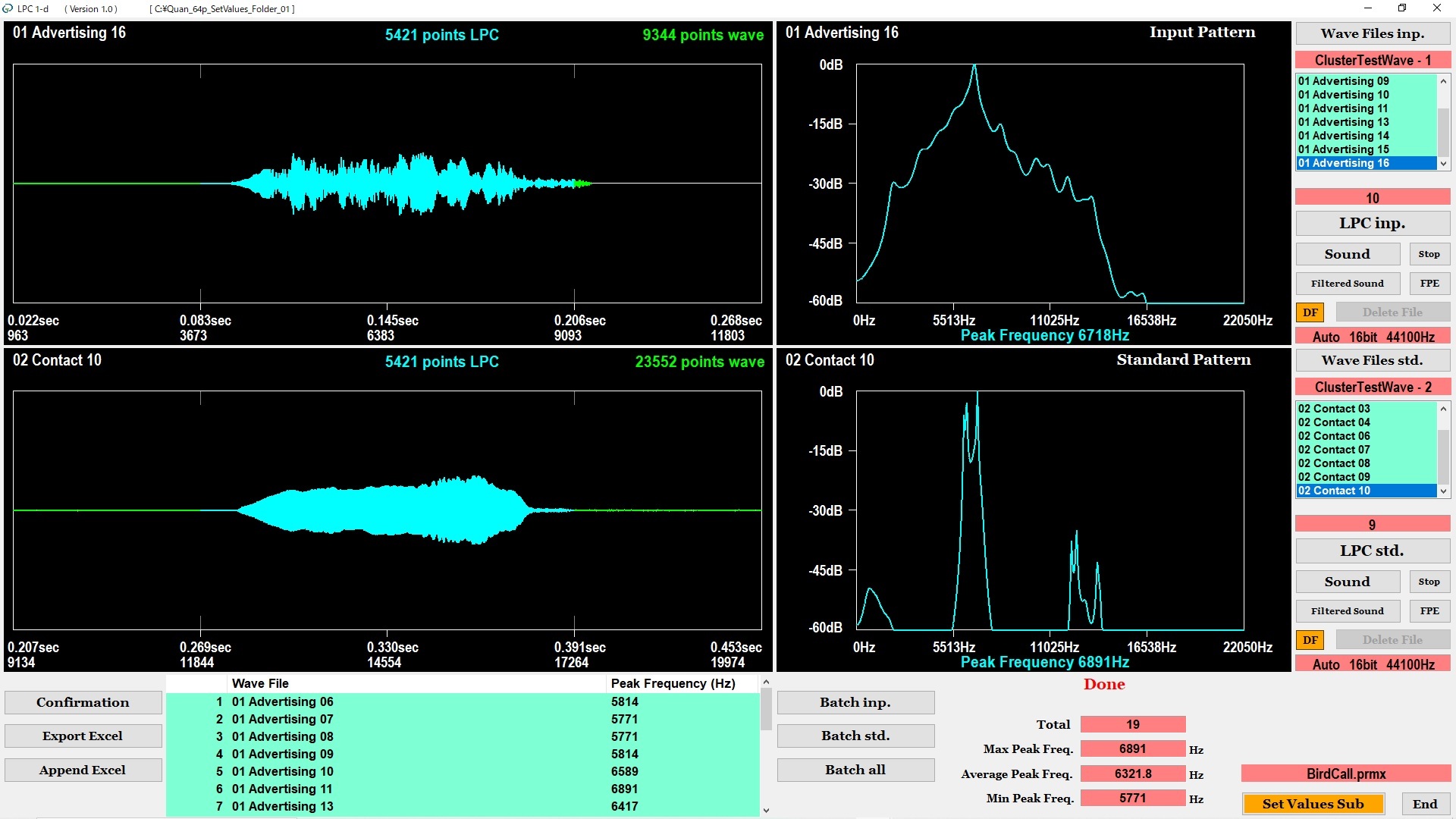
Figure 6. Oscillograms and One-dimensional LPC spectra
LPC 2-d
On the left of the screen shown in Figure 7, the software displays the oscillogram and the two-dimensional LPC spectrum of the WAV file that is selected from the first cluster. Similarly, on the right of the screen, the software displays the oscillogram and the two-dimensional LPC spectrum of the WAV file that is selected from the second cluster. Note that, the software displays the filtered oscillograms by the FIR digital filter, and extracts the two-dimensional LPC spectra from the cyan-colored waveforms, respectively. We can compare the two-dimensional LPC spectrum shown on the left of the screen with the two-dimensional LPC spectrum shown on the right of the screen. Furthermore, at the bottom of the screen, the software displays the list of the peak frequencies in the two-dimensional LPC spectra of all WAV files.

Figure 7. Oscillograms and Two-dimensional LPC spectra
Sonogram View
In the middle of the screen shown in Figure 8, the software displays the oscillogram and the sonogram of the WAV file that is selected from the cluster. Note that, the software displays the filtered oscillogram by the FIR digital filter, and extracts the sonogram from the cyan-colored waveform. The software has an enlargement display function, a scroll display function, a monochrome display function, and other functions. When the vertical red line is set in the middle of the screen using a computer mouse, on the right of the screen the software displays the cross-section of the sonogram in the position of the vertical red line as a one-dimensional LPC spectrum. Furthermore, in the window shown in Figure 9, the software displays the FPE (Final Prediction Error) and the AIC (Akaike Information Criterion) of the one-dimensional LPC spectrum.
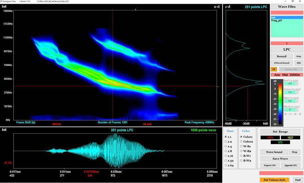
Figure 8. Oscillogram and Sonogram
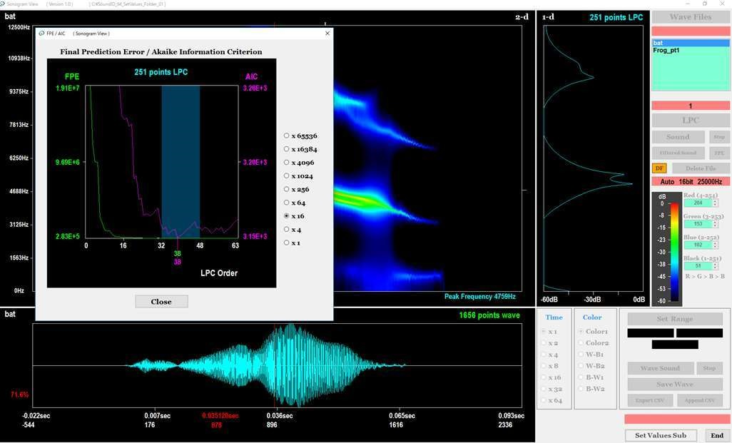
Figure 9. FPE and AIC
Users can arbitrarily specify frequency resolution Δf in the LPC spectrum.
Because the software displays the LPC spectrum using 697 pixels on the screen,
the frequency resolution Δf is calculated as follows.
(Example 1)
If LPC Freq.2 = 60000Hz (upper limit frequency on the screen) and
LPC Freq.1 = 40000Hz (lower limit frequency on the screen),
then frequency resolution Δf = ( 60000Hz – 40000Hz )/( 697 – 1 ) = 28.74Hz
(Example 2)
If LPC Freq.2 = 52000Hz (upper limit frequency on the screen) and
LPC Freq.1 = 48000Hz (lower limit frequency on the screen),
then frequency resolution Δf = ( 52000Hz – 48000Hz )/( 697 – 1 ) = 5.75Hz
Segmentation
On the screen shown in Figure 10, the software displays the result of the segmentation that segments waveforms of the target sound automatically from a continuous recording. We can confirm the result of the segmentation for the one-dimensional LPC spectrum, the two-dimensional LPC spectrum and the sonogram. In order to reduce the processing overhead, the recognition software does not display the image shown in Figure 10. We can confirm the result of segmentation using the segmentation software. Figure 11 shows the result of segmentation in the case where the target sounds are close. In order to distinguish the target sounds that are close, the software displays the target sounds using two colors (magenta and cyan) alternately. The software extracts LPC spectra from the magenta waveforms and the cyan waveforms respectively.
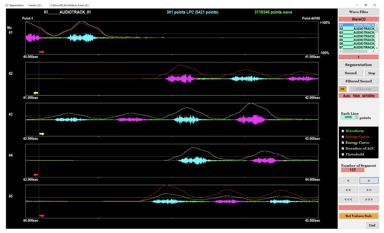
Figure 10. Segmentation of target sounds
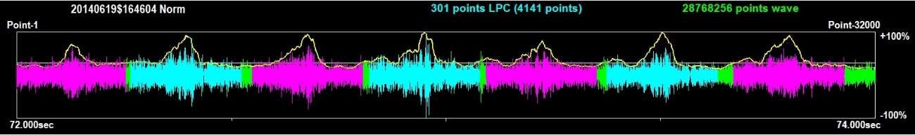
Figure 11. Segmentation of target sounds in close array
FIR Digital Filter
This is a simulation software for the FIR (Finite Impulse Response) digital filter. At the top right of the screen shown in Figure 12, we set “type of filter” and “characteristic values of filter”. At the bottom right of the screen, we set “sampling frequency” and “frequencies of two input waves”. These two input waves are added and input into the FIR digital filter. Figure 13 typically shows the relationship between the input wave (green) and the output wave (yellow) in FIR digital filter. At the top of the screen shown in Figure 12, the input waveform (green) and the output waveform (yellow) are displayed to overlap each other. Moreover, at the bottom of the screen shown in Figure 12, the linear transfer function or the logarithmic transfer function is displayed.

Figure 12. Input waveform, output waveform and transfer function in FIR digital filter
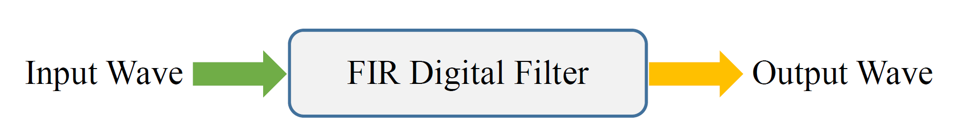
Figure 13. Input wave and output wave in FIR digital filter
Set Values Main
On the screen shown in Figure 14, we set the values for “FIR Digital Filter”, “Waveform”, “Segmentation”, “Linear Predictive Coefficient”, “Geometric Distance” and “Result”. We can “Save these values As” and “Open them”. Furthermore, we can “Save them As” and “Open them” in “LPC 1-d”, “LPC 2-d” and “Sonogram View”.
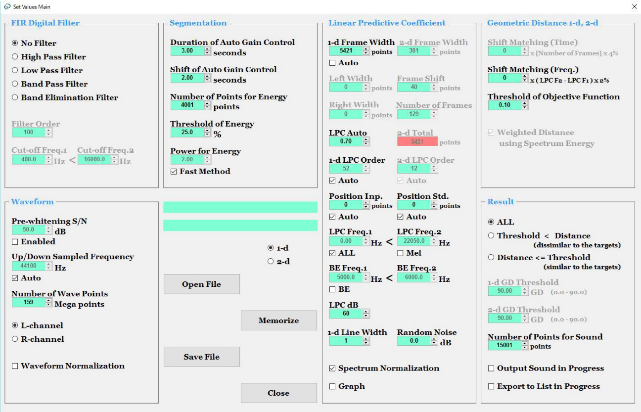
Figure 14. Parameter setting screen
LPC Spectrum Analyzer Basic specifications
FIR Digital Filter
| Types of Filter | No Filter / High Pass Filter / Low Pass Filter / Band Pass Filter / Band Elimination Filter |
|---|---|
| Filter Order | 3 to 10000 |
| Cut-off Frequencies 1 and 2 | 0.0 Hz to ( sampling frequency / 2.0 ) Hz |
Waveform
| Pre-whitening S/N | Disenabled / Enabled 0.0 dB to 9999.0 dB |
|---|---|
| Up/Down Sampled Frequency | Auto / Manual 0 to 99999999 |
| Number of Wave Points | 10 Mega points to 1073 Mega points |
| Channel Selection | L-channel / R-channel |
| Waveform Normalization | Disenabled / Enabled |
Segmentation
| Duration of Auto Gain Control | 0.05 seconds to 99999999.00 seconds |
|---|---|
| Shift of Auto Gain Control | 0.01 seconds to 99999999.00 seconds |
| Number of Points for Energy | 1 point to 99999999 points |
| Threshold | 0.0 % to 100.0 % |
| Power for Energy | P = 0.10 to 6.00 , where |W(t)|^P P = 1 when you select “Fast Method” |
Linear Predictive Coefficient
| 1-d Frame Width / 2-d Frame Width | 5 points to 9999999 points |
|---|---|
| Frame Shift | 1 points to 99999999 points |
| Number of Frames | 7 to 99999 |
| 1-d LPC Order / 2-d LPC Order | 3 to 30000 |
| Position Input / Position Standard | -999999999 to 999999999 |
| LPC Frequencies 1 and 2 | 0.0 Hz to ( sampling frequency / 2.0 ) Hz |
| Band Elimination Frequencies 1 and 2 | 0.0 Hz to ( sampling frequency / 2.0 ) Hz |
| LPC dB | 1 dB to 1000 dB |
| 1-d Line Width | 1 to 9 |
| Random Noise | 0.0 dB to 99999999.0 dB |
| Spectrum Normalization | Disenabled / Enabled |
| Graph in Progress | Disenabled / Enabled |
